Time series forecasting is a critical challenge in science and business, and recent innovations have brought deep learning models to the forefront alongside classical methods like ARIMA. A key distinction between these approaches lies in how they handle uncertainty and multiple time series.
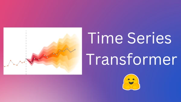
Unlike classical methods that fit each time series individually, deep learning enables training a global model on all available series, capturing latent patterns across diverse sources. This is especially valuable for probabilistic forecasting, which provides prediction uncertainties rather than single point estimates. By modeling a probabilistic distribution, decision-makers can sample forecasts and account for risk.
Deep neural networks naturally handle probabilistic forecasting by learning parameters of a distribution (e.g., Gaussian or Student-T) or by modeling quantiles. One can always convert a probabilistic model to a point forecast by taking the mean or median.
The Transformer for Time Series
The Transformer architecture, known for its success in NLP, is a strong fit for time series forecasting due to its sequential nature. The vanilla Transformer (Vaswani et al., 2017) serves as an encoder-decoder model for univariate probabilistic forecasting. At inference, it generates forecasts autoregressively, similar to text generation: given a context window, it samples from a distribution and feeds the prediction back into the decoder.
Transformers handle long sequences by using a context window, which is passed to the encoder, while the prediction window goes to a causal-masked decoder (teacher forcing). They can also naturally incorporate missing values via attention masks, avoiding explicit imputation.
However, the quadratic complexity of attention limits context and prediction window sizes, and the architecture's power increases the risk of overfitting.
Using the Time Series Transformer
The Hugging Face Transformers library now includes the Time Series Transformer. Below, we demonstrate how to train it on a custom dataset, using GluonTS for data preprocessing and batch creation.
First, install the required libraries: transformers, datasets, evaluate, accelerate, and gluonts.
!pip install -q transformers datasets evaluate accelerate gluonts ujson
We'll use the tourism_monthly dataset (Australian tourism volumes for 366 regions) from the Hugging Face Hub, part of the Monash Time Series Forecasting repository.
from datasets import load_dataset
dataset = load_dataset("monash_tsf", "tourism_monthly")
The dataset has three splits: train, validation, and test, with 366 time series each. Each example includes a start timestamp and target values.
print(dataset)
# DatasetDict({
#     train: Dataset({ features: ['start', 'target', 'feat_static_cat', 'feat_dynamic_real', 'item_id'], num_rows: 366 })
#     test: Dataset({ features: ['start', 'target', ...], num_rows: 366 })
#     validation: Dataset({ features: ['start', 'target', ...], num_rows: 366 })
# })
The next steps (not fully shown) involve data preprocessing, creating training batches, and fine-tuning the Time Series Transformer model. This approach paves the way for scalable and uncertainty-aware forecasting across many time series.